Trump vs Obama - a Battle of Words

Downloading Data

The twitteR library makes it easy to download tweets through the Twitter API. To access Twitter’s API you need to create a new app using Twitter Application Management. Once you have created an app, you can find the needed credentials in the “Keys and Access Tokens” tab. Now we can connect to the Twitter API using twitteR:

library(twitteR)

setup_twitter_oauth(
    consumer_key = Sys.getenv("TWITTER_CONSUMER_KEY"),
    consumer_secret = Sys.getenv("TWITTER_CONSUMER_SECRET"),
    access_token = Sys.getenv("TWITTER_ACCESS_TOKEN"),
    access_secret = Sys.getenv("TWITTER_ACCESS_SECRET")
)

## [1] "Using direct authentication"

After connecting to the API, downloading a user’s most recent tweets is a snap:

trump <- userTimeline('realDonaldTrump', n = 3200)
obama <- userTimeline('BarackObama', n = 3200)

Under the hood, the userTimeline() function is hitting the statuses/user_timeline API endpoint. “This method can only return up to 3,200 of a user’s most recent Tweets. Native retweets of other statuses by the user is included in this total, regardless of whether include_rts is set to false when requesting this resource.”

Cleaning Data

To start let’s create a data frame containing tweets by Donald Trump and Barack Obama.

library(tidyverse)

raw_tweets <- bind_rows(twListToDF(trump), twListToDF(obama))

The tidytext library makes cleaning text data a breeze. Let’s create a long data set with one row for each word from each tweet:

library(tidytext)

words <- raw_tweets %>%
    unnest_tokens(word, text)

Let’s remove common stop words:

data("stop_words")

words <- words %>%
    anti_join(stop_words, by = "word")

Let’s also remove some additional words I’d like to ignore:

options(stringsAsFactors = FALSE)

words_to_ignore <- data.frame(word = c("https", "amp", "t.co"))

words <- words %>%
    anti_join(words_to_ignore, by = "word")

Now let’s create a wide data set that has one row for each tweet and a column for each word. We will use this data to see which words best predict authorship.

tweets <- words %>%
    group_by(screenName, id, word) %>%
    summarise(contains = 1) %>%
    ungroup() %>%
    spread(key = word, value = contains, fill = 0) %>%
    mutate(tweet_by_trump = as.integer(screenName == "realDonaldTrump")) %>%
    select(-screenName, -id)

Modeling Authorship

Our data set has 594 rows (tweets) and 2213 columns (1 column indicating the author of the tweet and 2212 additional columns indicating whether a particular word was used in this tweet). Which words are most useful in predicting who authored a tweet? Lasso regression can help us determine which words are most predictive. The glmnet library makes it super easy to perform lasso regression:

library(glmnet)

fit <- cv.glmnet(
    x = tweets %>% select(-tweet_by_trump) %>% as.matrix(),
    y = tweets$tweet_by_trump,
    family = "binomial"
)

Let’s see which words have the largest coefficients:

temp <- coef(fit, s = exp(-3)) %>% as.matrix()
coefficients <- data.frame(word = row.names(temp), beta = temp[, 1])
data <- coefficients %>%
    filter(beta != 0) %>%
    filter(word != "(Intercept)") %>%
    arrange(desc(beta)) %>%
    mutate(i = row_number())

ggplot(data, aes(x = i, y = beta, fill = ifelse(beta > 0, "Trump", "Obama"))) +
    geom_bar(stat = "identity", alpha = 0.75) +
    scale_x_continuous(breaks = data$i, labels = data$word, minor_breaks = NULL) +
    xlab("") +
    ylab("Coefficient Estimate") +
    coord_flip() +
    scale_fill_manual(
        guide = guide_legend(title = "Word typically used by:"),
        values = c("#446093", "#bc3939")
    ) +
    theme_bw() +
    theme(legend.position = "top")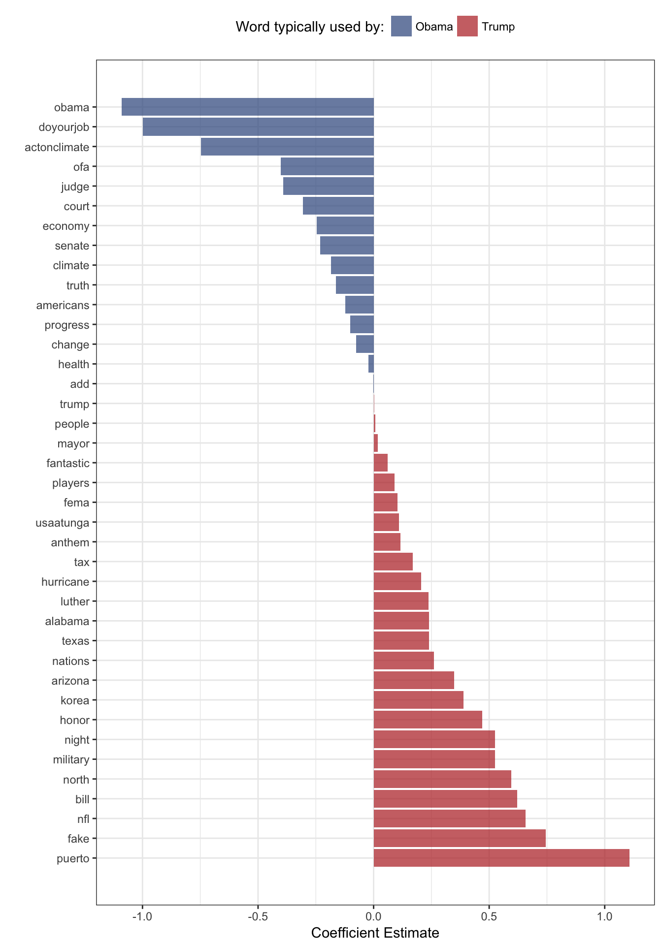

Word Clouds

The wordcloud library makes it super easy to make word clouds! Let’s make one for Trump:

library(wordcloud)

words %>%
    filter(screenName == "realDonaldTrump") %>%
    count(word) %>%
    with(wordcloud(word, n, max.words = 20))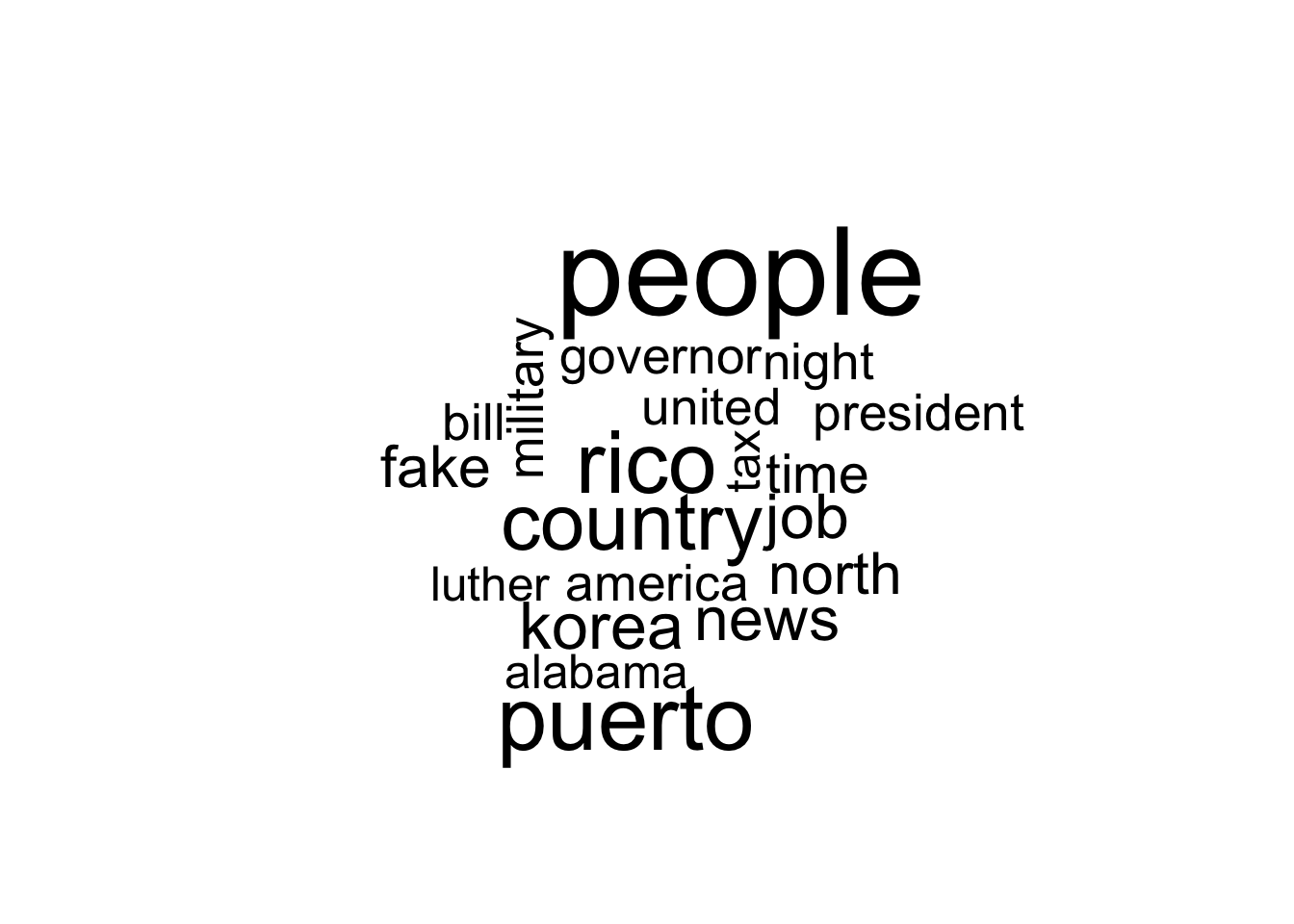

And one for Obama:

words %>%
    filter(screenName == "BarackObama") %>%
    count(word) %>%
    with(wordcloud(word, n, max.words = 20))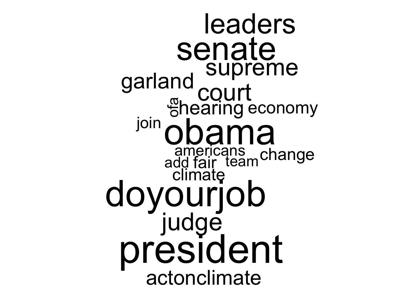

Warning

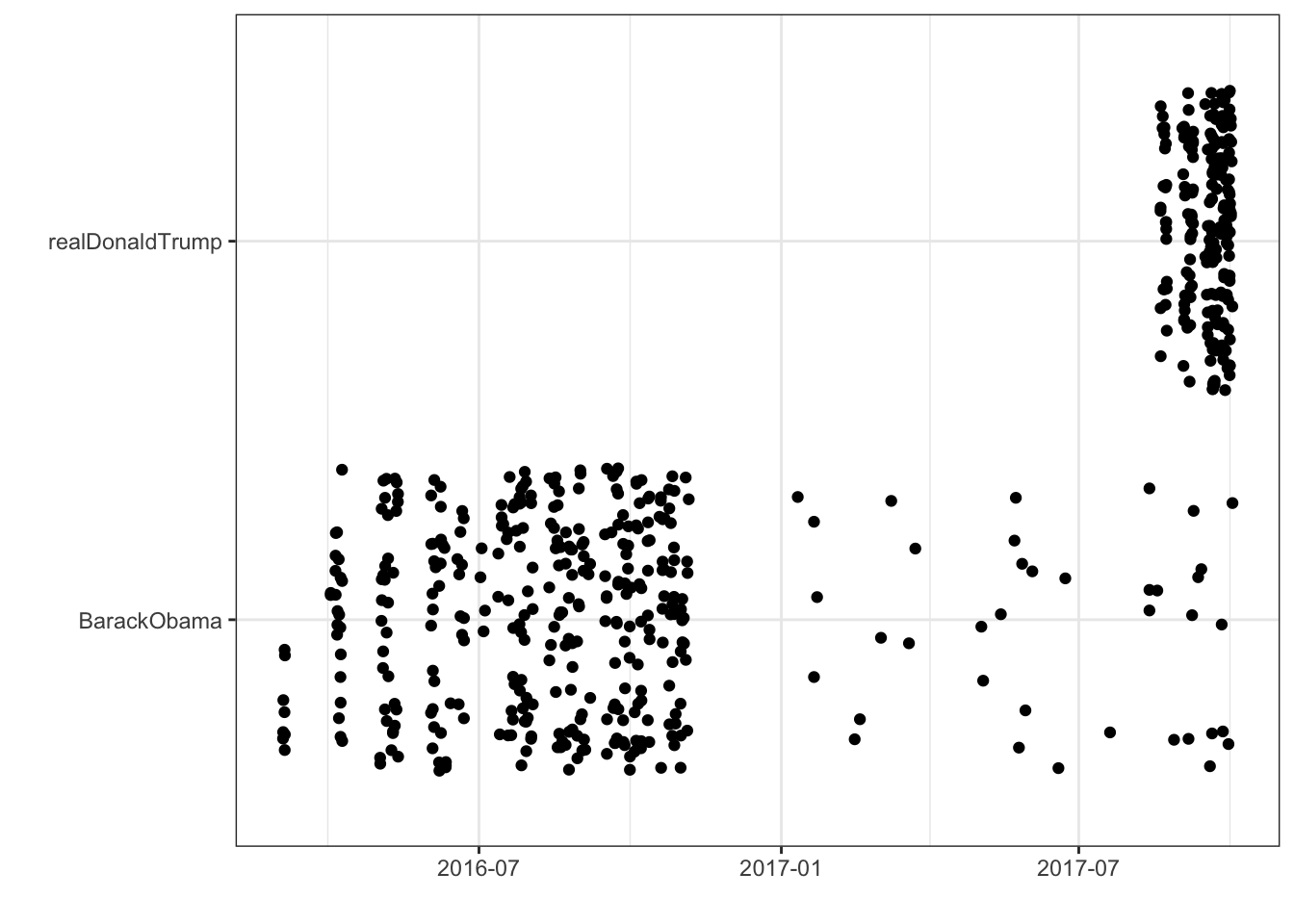
It looks like most of Barack Obama’s tweets are from 2016, while Donald Trump’s tweets have been more recent:

ggplot(raw_tweets, aes(x = created, y = screenName)) +
    geom_jitter(width = 0) +
    theme_bw() +
    ylab("") +
    xlab("")