Stata Tutorial
Stata is a commonly used tool for empirical research. Stata comes with an extensive library of statistical methods, and there are additional user written methods that extend the functionality of Stata even further.
Stata stores data in memory as a single matrix. If you are familiar with Microsoft Excel Workbooks, Stata stores a single Worksheet in memory where each column has a name and each row is numbered from 1 to the total number of rows in the dataset.
This tutorial aims to introduce you to the key features of Stata and its documentation so you can start your own empirical work.
Typing Commands
The display command is useful for showing values at the command
line.
. display 1 + 2
3
Use the Page Up key to recall the previous command evaluated. This
is particularly useful if you need to fix a typo.
Commands can be abbreviated, di is equivalent to display. I
prefer to use the whole command name because it makes code explicit.
Getting Help
Use the help command if you know the name of the function and want
more details. Use the findit command if you want to find a
function. I end up using Google more than findit, but this may be a
mistake.
Unfortunately the help command opens a new window each time you use
it, use the nonew option to prevent this behavior,
help help, nonew.
Reading Data Into Stata
There are many different ways to read data into Stata. To get a good
overview of how to import data into Stata type help import in
Stata’s Command window. The functions I use most are import excel
and insheet. import excel is great if you are working with an
Excel workbook, while insheet is great if you have a comma-separated
values (csv) file.
Stata datasets are generally stored in files with a .dta extension.
To read a Stata dataset use the use command. For the purpose of
this tutorial we will use a dataset shipped with Stata about
automobiles. Type in sysuse auto to load the dataset into memory.
. sysuse auto, clear
(1978 Automobile Data)
Descriptive Statistics
The describe command gives useful information about the variables in
the dataset and the number of rows in the dataset.
. describe

Contains data from /Applications/Stata/ado/base/a/auto.dta
  obs:            74                          1978 Automobile Data
 vars:            12                          13 Apr 2011 17:45
 size:         3,182                          (_dta has notes)
--------------------------------------------------------------------------------------------------------
              storage  display     value
variable name   type   format      label      variable label
--------------------------------------------------------------------------------------------------------
make            str18  %-18s                  Make and Model
price           int    %8.0gc                 Price
mpg             int    %8.0g                  Mileage (mpg)
rep78           int    %8.0g                  Repair Record 1978
headroom        float  %6.1f                  Headroom (in.)
trunk           int    %8.0g                  Trunk space (cu. ft.)
weight          int    %8.0gc                 Weight (lbs.)
length          int    %8.0g                  Length (in.)
turn            int    %8.0g                  Turn Circle (ft.)
displacement    int    %8.0g                  Displacement (cu. in.)
gear_ratio      float  %6.2f                  Gear Ratio
foreign         byte   %8.0g       origin     Car type
--------------------------------------------------------------------------------------------------------
Sorted by:  foreign
The summarize command gives some useful summary statistics for each
variable.
. summarize

    Variable |       Obs        Mean    Std. Dev.       Min        Max
-------------+--------------------------------------------------------
        make |         0
       price |        74    6165.257    2949.496       3291      15906
         mpg |        74     21.2973    5.785503         12         41
       rep78 |        69    3.405797    .9899323          1          5
    headroom |        74    2.993243    .8459948        1.5          5
-------------+--------------------------------------------------------
       trunk |        74    13.75676    4.277404          5         23
      weight |        74    3019.459    777.1936       1760       4840
      length |        74    187.9324    22.26634        142        233
        turn |        74    39.64865    4.399354         31         51
displacement |        74    197.2973    91.83722         79        425
-------------+--------------------------------------------------------
  gear_ratio |        74    3.014865    .4562871       2.19       3.89
     foreign |        74    .2972973    .4601885          0          1
You’ll notice that 11 of 12 variables in the auto dataset are numeric
and the make variable is a string. To see what the make variable
looks like, we can list the first few observations.
. list make if _n <= 5

     +---------------+
     | make          |
     |---------------|
  1. | AMC Concord   |
  2. | AMC Pacer     |
  3. | AMC Spirit    |
  4. | Buick Century |
  5. | Buick Electra |
     +---------------+
To see if make uniquely identifies each row in the dataset we can
use the isid function.
. isid make
When isid says nothing the variable list does uniquely identify each
row. Are cars uniquely identified by their weight and length?
. duplicates report make

Duplicates in terms of make

--------------------------------------
   copies | observations       surplus
----------+---------------------------
        1 |           74             0
--------------------------------------

. duplicates report weight length

Duplicates in terms of weight length

--------------------------------------
   copies | observations       surplus
----------+---------------------------
        1 |           70             0
        2 |            4             2
--------------------------------------
Imagine we are interested in looking at how foreign and domestic cars
differ. As a first step, it would be good to examine some summary
statistics for foreign and domestic cars, the tabstat command makes
this fairly easy.
. tabstat price mpg weight length, by(foreign) stat(mean sd)

Summary statistics: mean, sd
  by categories of: foreign (Car type)

 foreign |     price       mpg    weight    length
---------+----------------------------------------
Domestic |  6072.423  19.82692  3317.115  196.1346
         |  3097.104  4.743297  695.3637  20.04605
---------+----------------------------------------
 Foreign |  6384.682  24.77273  2315.909  168.5455
         |  2621.915  6.611187  433.0035  13.68255
---------+----------------------------------------
   Total |  6165.257   21.2973  3019.459  187.9324
         |  2949.496  5.785503  777.1936  22.26634
--------------------------------------------------
You may have noticed from the output of the summarize command that
rep78 has 5 missing values. We can look at those observations using
the list command:
. list if missing(rep78)

     +---------------------------------------------------------------------------------------------+
  3. | make          |  price | mpg | rep78 | headroom | trunk | weight | length | turn | displa~t |
     | AMC Spirit    |  3,799 |  22 |     . |      3.0 |    12 |  2,640 |    168 |   35 |      121 |
     |---------------------------------------------------------------------------------------------|
     |                   gear_r~o                   |                    foreign                   |
     |                       3.08                   |                   Domestic                   |
     +---------------------------------------------------------------------------------------------+

     +---------------------------------------------------------------------------------------------+
  7. | make          |  price | mpg | rep78 | headroom | trunk | weight | length | turn | displa~t |
     | Buick Opel    |  4,453 |  26 |     . |      3.0 |    10 |  2,230 |    170 |   34 |      304 |
     |---------------------------------------------------------------------------------------------|
     |                   gear_r~o                   |                    foreign                   |
     |                       2.87                   |                   Domestic                   |
     +---------------------------------------------------------------------------------------------+

     +---------------------------------------------------------------------------------------------+
 45. | make          |  price | mpg | rep78 | headroom | trunk | weight | length | turn | displa~t |
     | Plym. Sapporo |  6,486 |  26 |     . |      1.5 |     8 |  2,520 |    182 |   38 |      119 |
     |---------------------------------------------------------------------------------------------|
     |                   gear_r~o                   |                    foreign                   |
     |                       3.54                   |                   Domestic                   |
     +---------------------------------------------------------------------------------------------+

     +---------------------------------------------------------------------------------------------+
 51. | make          |  price | mpg | rep78 | headroom | trunk | weight | length | turn | displa~t |
     | Pont. Phoenix |  4,424 |  19 |     . |      3.5 |    13 |  3,420 |    203 |   43 |      231 |
     |---------------------------------------------------------------------------------------------|
     |                   gear_r~o                   |                    foreign                   |
     |                       3.08                   |                   Domestic                   |
     +---------------------------------------------------------------------------------------------+

     +---------------------------------------------------------------------------------------------+
 64. | make          |  price | mpg | rep78 | headroom | trunk | weight | length | turn | displa~t |
     | Peugeot 604   | 12,990 |  14 |     . |      3.5 |    14 |  3,420 |    192 |   38 |      163 |
     |---------------------------------------------------------------------------------------------|
     |                   gear_r~o                   |                    foreign                   |
     |                       3.58                   |                    Foreign                   |
     +---------------------------------------------------------------------------------------------+
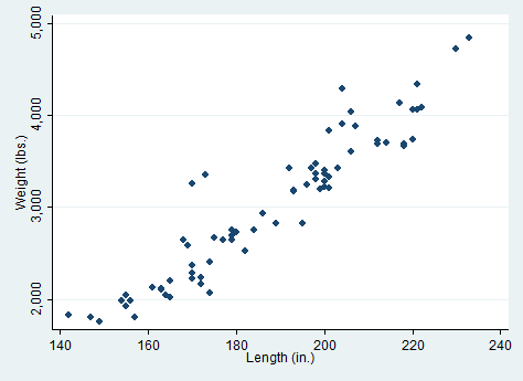
Graphs
There are good graph galleries provided by StataCorp, UCLA, and Survey Design and Analysis Services. Below is a simple scatter plot of weight versus length:
. graph twoway scatter weight length

. graph export scatter.png, replace
(file scatter.png written in PNG format)
Creating New Variables
There are a number of ways to create new variables or modifying
existing variables. The most important command in this section is the
generate command. Imagine we are curious about cars that are heavy
for their length we could create a new variable
. generate weight_per_length = weight / length
This creates a new column in the dataset, for each car we have calculated the ratio of that car’s weight to its length. Let’s take a look at the top five heaviest cars per length.
. gsort -weight_per_length

. list make weight_per_length if _n <= 5

     +------------------------------+
     | make                weight~h |
     |------------------------------|
  1. | Cad. Seville        21.02941 |
  2. | Linc. Continental   20.77253 |
  3. | Linc. Mark V        20.52174 |
  4. | Cad. Deville        19.59276 |
  5. | Olds Toronado       19.56311 |
     +------------------------------+
Another very useful command for generating new variables is the egen
command. This is particularly useful is you want to merge summary
statistics for groups of cars back into the larger dataset. For
instance, we might be curious to see how a car’s price compares to the
average price among foreign or domestic cars. We can find the average
price for foreign and domestic cars using tabstat, but how do we make
a column in the dataset with these values?
. tabstat price, by(foreign)

Summary for variables: price
     by categories of: foreign (Car type)

 foreign |      mean
---------+----------
Domestic |  6072.423
 Foreign |  6384.682
---------+----------
   Total |  6165.257
--------------------

. egen ave_price = mean(price), by(foreign)

. list foreign ave_price

     +---------------------+
     |  foreign   ave_pr~e |
     |---------------------|
  1. | Domestic   6072.423 |
  2. | Domestic   6072.423 |
  3. | Domestic   6072.423 |
  4. | Domestic   6072.423 |
  5. | Domestic   6072.423 |
     |---------------------|
  6. | Domestic   6072.423 |
  7. | Domestic   6072.423 |
  8. | Domestic   6072.423 |
  9. | Domestic   6072.423 |
 10. | Domestic   6072.423 |
     |---------------------|
 11. | Domestic   6072.423 |
 12. | Domestic   6072.423 |
 13. | Domestic   6072.423 |
 14. | Domestic   6072.423 |
 15. |  Foreign   6384.682 |
     |---------------------|
 16. | Domestic   6072.423 |
 17. | Domestic   6072.423 |
 18. | Domestic   6072.423 |
 19. | Domestic   6072.423 |
 20. | Domestic   6072.423 |
     |---------------------|
 21. | Domestic   6072.423 |
 22. | Domestic   6072.423 |
 23. | Domestic   6072.423 |
 24. | Domestic   6072.423 |
 25. | Domestic   6072.423 |
     |---------------------|
 26. | Domestic   6072.423 |
 27. | Domestic   6072.423 |
 28. | Domestic   6072.423 |
 29. | Domestic   6072.423 |
 30. | Domestic   6072.423 |
     |---------------------|
 31. | Domestic   6072.423 |
 32. | Domestic   6072.423 |
 33. | Domestic   6072.423 |
 34. | Domestic   6072.423 |
 35. |  Foreign   6384.682 |
     |---------------------|
 36. | Domestic   6072.423 |
 37. | Domestic   6072.423 |
 38. | Domestic   6072.423 |
 39. | Domestic   6072.423 |
 40. | Domestic   6072.423 |
     |---------------------|
 41. | Domestic   6072.423 |
 42. | Domestic   6072.423 |
 43. | Domestic   6072.423 |
 44. |  Foreign   6384.682 |
 45. | Domestic   6072.423 |
     |---------------------|
 46. | Domestic   6072.423 |
 47. |  Foreign   6384.682 |
 48. |  Foreign   6384.682 |
 49. |  Foreign   6384.682 |
 50. | Domestic   6072.423 |
     |---------------------|
 51. | Domestic   6072.423 |
 52. |  Foreign   6384.682 |
 53. |  Foreign   6384.682 |
 54. | Domestic   6072.423 |
 55. |  Foreign   6384.682 |
     |---------------------|
 56. | Domestic   6072.423 |
 57. |  Foreign   6384.682 |
 58. |  Foreign   6384.682 |
 59. |  Foreign   6384.682 |
 60. | Domestic   6072.423 |
     |---------------------|
 61. |  Foreign   6384.682 |
 62. | Domestic   6072.423 |
 63. | Domestic   6072.423 |
 64. |  Foreign   6384.682 |
 65. |  Foreign   6384.682 |
     |---------------------|
 66. |  Foreign   6384.682 |
 67. |  Foreign   6384.682 |
 68. |  Foreign   6384.682 |
 69. |  Foreign   6384.682 |
 70. | Domestic   6072.423 |
     |---------------------|
 71. |  Foreign   6384.682 |
 72. |  Foreign   6384.682 |
 73. |  Foreign   6384.682 |
 74. | Domestic   6072.423 |
     +---------------------+
Regressions
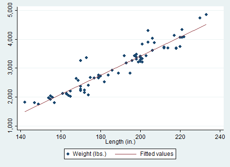
To further explore the relationship between weight and length we can run a regression.
. regress weight length

      Source |       SS       df       MS              Number of obs =      74
-------------+------------------------------           F(  1,    72) =  613.27
       Model |  39461306.8     1  39461306.8           Prob > F      =  0.0000
    Residual |  4632871.55    72  64345.4382           R-squared     =  0.8949
-------------+------------------------------           Adj R-squared =  0.8935
       Total |  44094178.4    73  604029.841           Root MSE      =  253.66

------------------------------------------------------------------------------
      weight |      Coef.   Std. Err.      t    P>|t|     [95% Conf. Interval]
-------------+----------------------------------------------------------------
      length |   33.01988   1.333364    24.76   0.000     30.36187    35.67789
       _cons |  -3186.047   252.3113   -12.63   0.000     -3689.02   -2683.073
------------------------------------------------------------------------------
We see that on average, each additional inch is associated with 33 pounds. We can plot the predicted values from the regression on the scatter plot from above.
. graph twoway (scatter weight length) (lfit weight length)

. graph export scatter_lfit.png, replace
(file scatter_lfit.png written in PNG format)
Further Reading
Germán Rodríguez’s Stata Tutorial is an excellent introduction to Stata..
These notes on writing code by Matthew Gentzkow and Jesse Shapiro have excellent suggestions on how to program with Stata.