Republican vs Democrat - Searching for Middle Ground
Can we find topics where Democrats and Republicans agree? This post aims to find political middle ground using natural language processing and machine learning. Examining tweets by party leaders in the House and Senate, I fit a neural network based on the words used in each tweet to predict the political party of each tweet’s author. By examining tweets where the neural network has a hard time predicting the author’s political party I hope to identify a political middle ground (tweets where the word choice is not obviously partisan).
Download Data
Let’s download the most recent tweets by the party leaders in Congress.
library(twitteR)
library(tidyverse)

party_leaders <- read_csv(trimws('
name            , party , position , chamber , username
Kevin McCarthy  , R     , Leader   , House   , GOPLeader
Nancy Pelosi    , D     , Leader   , House   , NancyPelosi
Steve Scalise   , R     , Whip     , House   , SteveScalise
Steny Hoyer     , D     , Whip     , House   , WhipHoyer
Mitch McConnell , R     , Leader   , Senate  , SenateMajLdr
Chuck Schumer   , D     , Leader   , Senate  , SenSchumer
John Cornyn     , R     , Whip     , Senate  , JohnCornyn
Dick Durbin     , D     , Whip     , Senate  , SenatorDurbin
'))

read_tweets <- function(users) {
    # Connect to the Twitter API
    capture.output(setup_twitter_oauth(
        consumer_key = Sys.getenv("TWITTER_CONSUMER_KEY"),
        consumer_secret = Sys.getenv("TWITTER_CONSUMER_SECRET"),
        access_token = Sys.getenv("TWITTER_ACCESS_TOKEN"),
        access_secret = Sys.getenv("TWITTER_ACCESS_SECRET")
    ))

    # Download tweets
    l <- lapply(users, function(user) twListToDF(userTimeline(user, n = 3200)))

    # Create a data frame of tweets
    tweets <- do.call(bind_rows, l)
    return(tweets)
}

tweets <- read_tweets(party_leaders$username)
tweets <- tweets %>%
    left_join(party_leaders, by = c("screenName" = "username")) %>%
    mutate(republican = as.integer(party == "R"))
Clean Data
Select Time Period
Twitter’s API let’s us download a user’s most recent tweets (3,200 minus retweets). The graph below illustrates when each tweet in our dataset was posted.
ggplot(tweets, aes(x = created, y = paste0(name, " (", party, ")"))) +
    geom_jitter(width = 0, size = 0.5) +
    theme_bw() +
    ylab("") +
    xlab("")
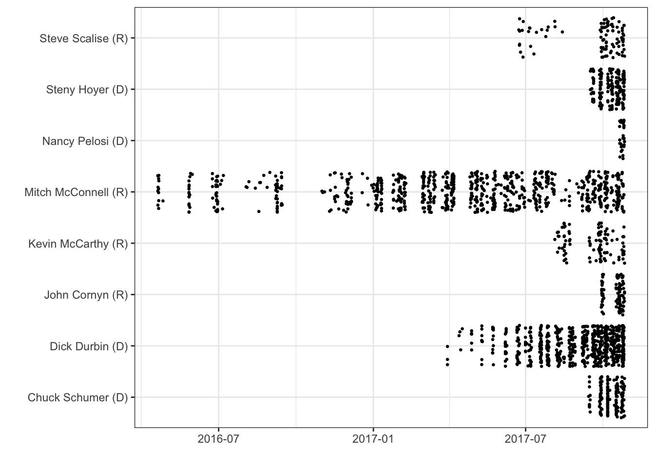
I want to make sure we focus on an overlapping time period so our model doesn’t pick up on unique words in Mitch McConnell’s early tweets.
common_time_period <- function(tweets) {
    x <- tweets %>%
        group_by(republican) %>%
        summarise(first = min(created))
    start <- max(x$first)
    cat("I restrict the analysis to tweets since ", as.character(start), ".", sep = "")

    tweets %>%
        filter(created >= start)
}

tweets <- common_time_period(tweets)
I restrict the analysis to tweets since 2017-03-30 01:06:54.
Convert Text to Numbers
I use the tidytext library to create dummy variables indicating whether a word was used in a given tweet.
library(tidytext)
library(rlang)

expand_text_into_dummy_variables <- function(.data, text_column, id_column, cutoff, ignore) {
    id_column <- enquo(id_column)
    text_column <- enquo(text_column)

    .data <- .data %>% select(-starts_with("word_"))

    data("stop_words")
    words_to_ignore <- data.frame(word = ignore, stringsAsFactors = FALSE)

    words <- .data %>%
        unnest_tokens(output = word, input = !!text_column) %>%
        anti_join(stop_words, by = "word") %>%
        anti_join(words_to_ignore, by = "word")

    N <- nrow(.data)
    freq <- words %>%
        group_by(word) %>%
        summarise(n = length(unique(!!id_column))) %>%
        mutate(pct = n / N)

    filtered <- freq %>%
        filter(pct >= cutoff)

    words <- words %>%
        inner_join(filtered, by = "word")

    dummies <- words %>%
        group_by(!!id_column, word) %>%
        summarise(contains = 1) %>%
        ungroup() %>%
        spread(key = word, value = contains, fill = 0, sep = "_")

    l <- sapply(colnames(dummies), function(i) 0)

    .data %>%
        full_join(dummies, by = f_text(id_column)) %>%
        replace_na(replace = as.list(l))
}

tweets <- tweets %>%
    expand_text_into_dummy_variables(
        text_column = text, id_column = id, cutoff = 0.015,
        ignore = c("https", "t.co", "amp", "1", "2", "2015", "it’s")
    )
After dropping stop words and focusing on words that appear in at least 1.5% of all tweets, we’re left with 68 words. For each of these 68 words I’ve created a new dummy variable indicating which tweets contain this word.
Model Authorship
I want to build a neural network to predict the political party of a tweet’s author. Let’s fit a neural network with two hidden states.
library(nnet)

tweets <- tweets %>%
    group_by(screenName) %>%
    mutate(weight = 1 / n()) %>%
    ungroup()

expvars <- function(data) {
    data %>%
        select(starts_with("word_")) %>%
        as.matrix()
}

set.seed(1)
fit <- nnet(
    y = tweets$republican,
    x = expvars(tweets),
    weights = tweets$weight,
    size = 2,
    maxit = 5000
)
And save its predictions in a variable named yhat.
tweets$yhat <- predict(fit, expvars(tweets))[, 1]
Evaluate Predictions
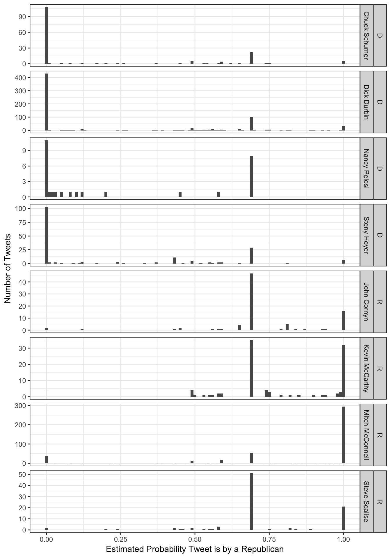
Let’s see how well our neural network predicts the political party associated with each tweet based on the words used.
tweets %>%
    ggplot(aes(x = yhat)) +
    geom_histogram(binwidth = 0.01) +
    facet_grid(party + name ~ ., scales = "free_y") +
    theme_bw() +
    xlab("Estimated Probability Tweet is by a Republican") +
    ylab("Number of Tweets")
tweets <- tweets %>%
    mutate(correct = (republican & (yhat > 0.5)) | (!republican & (yhat < 0.5)))
The model accurately predicts the political party of 78% of tweets.
Interpret Neural Network
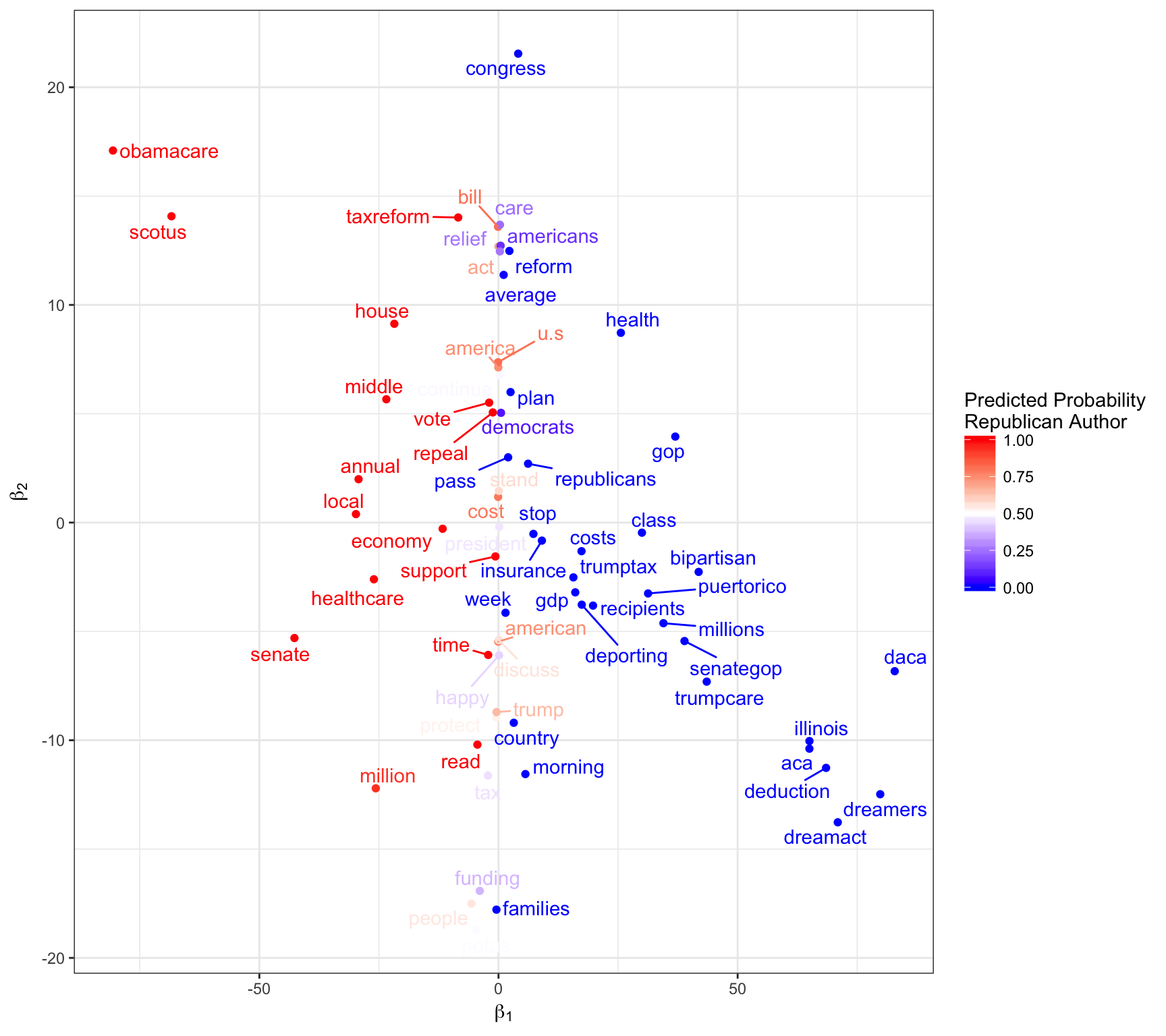
The plot below embeds the 68 words extracted from the 1823 tweets in a two-dimensional space. The x- and y-coordinates are edge weights from the neural network. The x-coordinate reports the weight from the node indicating the word was included in the tweet to the first hidden node. The y-coordinate reports the weight from the input word to the second hidden node. I have colored each word based on the probability a tweet containing only that word would be authored by a Republican. A tweet about “obamacare” is likely written by a Republican, while a tweet about “dreamers” is likely written by a Democrat.
library(ggrepel)

my_coef <- function(object) {
    x <- data.frame(coefficient = coef(object))
    x$edge <- row.names(x)
    row.names(x) <- NULL
    x %>%
        separate(col = "edge", into = c("source", "destination"), sep = "->")
}

plot_nnet <- function(fit, tweets) {
    beta <- my_coef(fit)

    words <- grep("word_", colnames(tweets), value = TRUE)
    labels <- data.frame(
        source = paste0("i", 1:length(words)),
        label = sub("word_", "", words)
    )
    x <- data.frame(variable = words, i = 1:length(words), value = 1) %>%
        spread(variable, value, fill = 0)

    labels$yhat <- predict(fit, newdata = x %>% select(starts_with("word_")))

    beta2 <- beta %>% inner_join(labels, by = "source") %>%
        select(-source) %>%
        spread(key = destination, value = coefficient)

    ggplot(beta2, aes(x = h1, y = h2, label = label, color = yhat)) +
        geom_point() +
        geom_text_repel() +
        scale_colour_gradientn(colours = c("blue", "white", "red"),
                               values = c(0, 0.5, 1), name = "Predicted Probability\nRepublican Author") +
        theme_bw() +
        xlab(expression(beta[1])) +
        ylab(expression(beta[2]))
}

plot_nnet(fit, tweets)
Inspect Middle Ground
For each of the eight politicians studied let’s look at his or her most central tweet (a tweet is central when its predicted probability is close to 50%).
middle_ground <- tweets %>%
    mutate(d = abs(yhat - 0.5)) %>%
    group_by(screenName) %>%
    arrange(d) %>%
    do(head(., 1)) %>%
    mutate(shortcodes = paste0("{{", "< tweet ", id, " >", "}}"))

for (shortcode in middle_ground$shortcodes) {
    cat("1.  ", shortcode, "\n\n")
}
.@POTUS & @IvankaTrump's #STEM initiative will help ensure future generations of American workers are job-ready on day one. 🇺🇸 pic.twitter.com/9ahbDpeGH2
— Kevin McCarthy (@GOPLeader) September 25, 2017Why should federal taxpayers subsidize high-tax states? https://t.co/JteXqlk9cx via @WSJ
— Senator John Cornyn (@JohnCornyn) October 24, 2017#GOPBudget borrows from our children's future to give massive tax cuts to the rich.
— Nancy Pelosi (@NancyPelosi) October 25, 2017.@POTUS is not getting nearly enough credit for the work he is doing to reshape our courts and commissions. pic.twitter.com/UsMTJQYvv3
— Leader McConnell (@SenateMajLdr) October 23, 2017.@POTUS playing politics with contraceptive coverage is an attack on American women, plain and simple. https://t.co/s5g5sx9Gv1
— Senator Dick Durbin (@SenatorDurbin) October 6, 2017.@POTUS promised to crackdown on China - so far it's been a lot of talk. @SenateDems say enough. Let's put US steel & aluminium jobs first. pic.twitter.com/4uvey9gCbp
— Chuck Schumer (@SenSchumer) October 23, 2017Today, @POTUS awarded the Medal of Valor to the heroes who saved the lives of everyone at the baseball field on June 14. pic.twitter.com/xgOV32fp7c
— Rep. Steve Scalise (@SteveScalise) July 27, 2017.@POTUS is shortening open enrollment—be sure to visit https://t.co/OqCEr7DFhC between Nov. 1-Dec. 15 to sign up for coverage. RT to share. pic.twitter.com/ops0LtDKQ7
— Steny Hoyer (@WhipHoyer) October 25, 2017
I wouldn’t classify this as a resounding success, but I think it shows some promise. The tweets by Kevin McCarthy and Steve Scalise seem close to a middle ground where the party of the author is not completely obvious to a human reader. I think the next step would be to improve the predictive model - make the robot better at reading political tweets.